Context
The term “uncertainty” refers to the necessary discrepancies between the mathematical model of a physical system, and the reality. Such uncertainties may degrade the stability or the performance of the system, and motivate for robustness considerations as of the control design. In particular, one can distinguish the unstructured uncertainties, which translate all kinds of neglected dynamics such as high-frequency dynamics or non-linearities, from the structured, or parametric, uncertainties, where a parameter is known only to the extent that it lies in some bounded interval. Parametric uncertainties are common in real-world applications; they can arise, for example, from manufacturing or measuring errors, variable operating conditions, time-varying characteristics, or inherent modeling limitations.
Mathematical representation
In the SDTlib, and more generally in the framework of linear robust control, parametric (structured) uncertainties are addressed with the Linear Fractional Transformations (LFT) framework [ZDG96]. The nominal state-space representation reads:
\begin{equation}
\left\lbrace \begin{array}{l}
\mathbf{\dot x} = \mathbf A \mathbf x + \mathbf B \mathbf u \\
\mathbf y = \mathbf C \mathbf x + \mathbf D \mathbf u
\end{array}
\right.
\end{equation}
Where $\mathbf x$ is the state vector, $\mathbf u$ is the input vector, $\mathbf y$ is the output vector, and the matrices A, B, C, D have appropriate dimensions. In the uncertain state-space representation, these matrices depend on a set of uncertain parameters $\delta_i$ :
\begin{equation}
\left\lbrace \begin{array}{l}
\mathbf{\dot x} = \mathbf A(\delta_i) \mathbf x + \mathbf B(\delta_i) \mathbf u \\
\mathbf y = \mathbf C(\delta_i) \mathbf x + \mathbf D(\delta_i) \mathbf u
\end{array}
\right.
\end{equation}
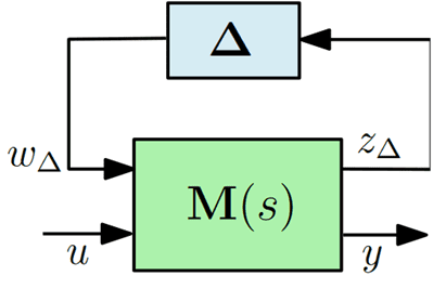
The LFT framework allows to rewrite this state-space representation under a form where the uncertainties are isolated from the nominal plant:
\begin{equation}
\left\lbrace \begin{array}{l}
\mathbf{\dot x} = \mathbf A \mathbf x + \mathbf B_1 \mathbf u + \mathbf B_2 \mathbf w_\Delta\\
\mathbf y = \mathbf C_1 \mathbf x + \mathbf D_{11} \mathbf u + \mathbf D_{12} \mathbf w_\Delta \\
\mathbf z_\Delta = \mathbf C_2\mathbf x + \mathbf D_{21} \mathbf u + \mathbf D_{22} \mathbf w_\Delta \\
\mathbf w = \Delta \mathbf z \\
\end{array}
\right.
\end{equation}
where the unknown, bounded matrix $\Delta = \mathrm{diag}(\delta_i \mathbf I_{n_i})$ (where $n_i$ is the number of occurrences of parameter $\delta_i$, and $\mathbf I_{n_i}$ is the identity matrix of size $n_i$) is expressed as a feedback of the nominal system. Next Figure represents the corresponding block-diagram, where $\mathbf M(\mathrm s)$ is the appropriate transfer matrix. Without loss of generality, since normalization operations can be integrated in the plant $\mathbf M(\mathrm s)$, it can be assumed that the $\delta_i$ verify $\mid \delta_i \mid < 1$.

Example
A mass m with ±10% of uncertainty can be represented as :
\begin{equation}
m = m_0 (1+0.1\delta)
\end{equation}
where $m_0$ is the nominal value, and $\delta$ is an unknown real number verifying $\mid \delta \mid < 1$. The block diagram is shown in next Figure:

In practice
Essentially, deriving an LFT model consists in finding a block-diagram representation of the system and “isolate the deltas”. In particular, it requires the matrices $\mathbf A(\delta_i)$, $\mathbf B(\delta_i)$, $\mathbf C(\delta_i)$, $\mathbf D(\delta_i)$ to be polynomial or rational functions of the parametric uncertainties $\delta_i$.
The LFT form allows representing the uncertain system with one single continuous model instead of a discrete family of parameterized models. It enables modern analysis and control tools such as the μ-analysis or the robust H infinity control, to ensure robust stability and performance to parametric uncertainties. In the SDTlib, parametric uncertainties may be the mass of an element, moment of inertia, natural frequency of a flexible body, position of a connection point of two elements…
References
[ZDG96] Kemin Zhou, John C Doyle, and Keith Glover. Robust and Optimal Control. Englewood Cliffs: Prentice hall, 1996.
